Projects > Deep Learning for Traffic Signs

Code for this project can be found on: Github.

I've also written about this project on Medium and Quora.

As part of completing the second project of Udacity's Self-Driving Car Engineer online course, I had to implement and train a deep neural network to identify German traffic signs. The following is a brief outline of the project:

The Dataset

In total, the dataset used is publicly accessible on this website and consisted of 51,839 RGB images with dimensions 32x32.

34,799 of the dataset images were used as a training dataset, 12,630 of the images were used as a testing dataset, and 4,410 of the images were used as a validation dataset.

A validation set was used to assess how well the model is performing. A low accuracy on the training and validation sets implies underfitting. A high accuracy on the training set but low accuracy on the validation set implies overfitting. The validation set was purely used to calibrate the network's hyperparameters.

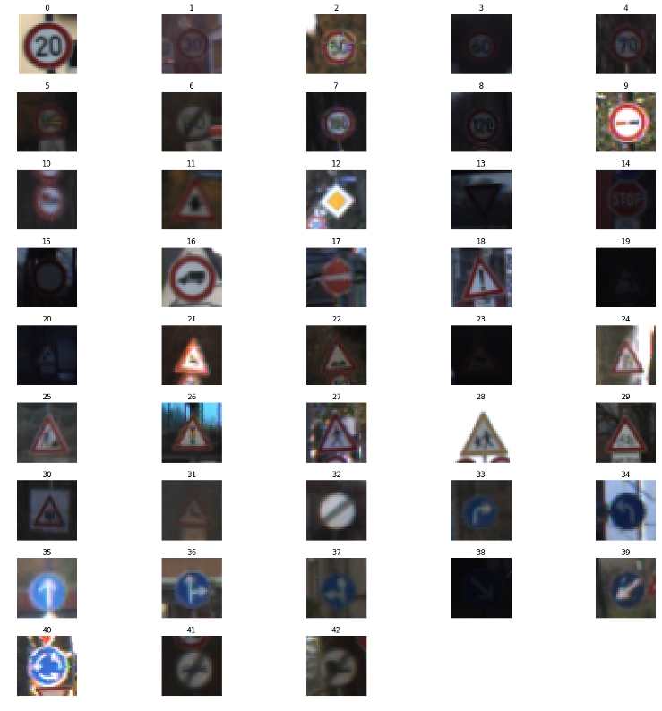
The dataset consisted of images belonging to 43 classes. Each class corresponds to a specific sign, for example, the class with label 4 represents 70km/h speed limit signs, and the class with label 25 represents a roadwork sign.

A sample from each class is shown in the image below:

The LeNet-5 Neural Network

The prediction model used for this project was a LeNet-5 deep neural network invented by Yann Lecun and further discussed on his website here. Yann has also published this paper on applying convolutional networks for traffic sign recognition, which was used as a reference.

The Tensorflow machine learning library was used to implement the LeNet-5 neural network. It consisted of the following layers:

Layer	Description
Input	32x32x3 RGB Image
Convolution 5x5	1x1 stride, valid padding, outputs 28x28x6
RELU	Rectified linear unit
Max Pooling	2x2 stride, outputs 16x16x6
Convolution 5x5	1x1 stride, valid padding, outputs 10x10x6
RELU	Rectified linear unit
Max Pooling	2x2 stride, outputs 5x5x16
Flatten	outputs 400
Fully connected	input 400, outputs 120
RELU	Rectified linear unit
Fully connected	input 120, outputs 84
RELU	Rectified linear unit
Fully connected	input 84, outputs 43

The pixel data of each image was normalized before it was fed into the neural network. The output of the neural network was also normalized using the softmax function to produce logits in the range [0, 1]. My choice for an activation function was a rectifier as it has been shown in a paper titled Deep Sparse Rectifier Neural Networks that they perform better than the sigmoid activation function for deep neural networks.

The following is the implementation of the above neural network in code:

    
import tensorflow as tf
from tensorflow.contrib.layers import flatten

def LeNet(x):
    mu = 0
    sigma = 0.1

    # Layer 1: Convolutional. Input = 32x32x3. Output = 28x28x6.
    conv1_W = tf.Variable(tf.truncated_normal(shape=(5, 5, 3, 6), mean = mu, stddev = sigma))
    conv1_b = tf.Variable(tf.zeros(6))
    conv1   = tf.nn.conv2d(x, conv1_W, strides=[1, 1, 1, 1], padding='VALID') + conv1_b

    # Activation.
    conv1 = tf.nn.relu(conv1)

    # Pooling. Input = 28x28x6. Output = 14x14x6.
    conv1 = tf.nn.max_pool(conv1, ksize=[1, 2, 2, 1], strides=[1, 2, 2, 1], padding='VALID')

    # Layer 2: Convolutional. Output = 10x10x16.
    conv2_W = tf.Variable(tf.truncated_normal(shape=(5, 5, 6, 16), mean = mu, stddev = sigma))
    conv2_b = tf.Variable(tf.zeros(16))
    conv2   = tf.nn.conv2d(conv1, conv2_W, strides=[1, 1, 1, 1], padding='VALID') + conv2_b

    # Activation.
    conv2 = tf.nn.relu(conv2)

    # Pooling. Input = 10x10x16. Output = 5x5x16.
    conv2 = tf.nn.max_pool(conv2, ksize=[1, 2, 2, 1], strides=[1, 2, 2, 1], padding='VALID')

    # Flatten. Input = 5x5x16. Output = 400.
    fc0   = flatten(conv2)

    # Layer 3: Fully Connected. Input = 400. Output = 120.
    fc1_W = tf.Variable(tf.truncated_normal(shape=(400, 120), mean = mu, stddev = sigma))
    fc1_b = tf.Variable(tf.zeros(120))
    fc1   = tf.matmul(fc0, fc1_W) + fc1_b

    # Activation.
    fc1    = tf.nn.relu(fc1)

    # Layer 4: Fully Connected. Input = 120. Output = 84.
    fc2_W  = tf.Variable(tf.truncated_normal(shape=(120, 84), mean = mu, stddev = sigma))
    fc2_b  = tf.Variable(tf.zeros(84))
    fc2    = tf.matmul(fc1, fc2_W) + fc2_b

    # Activation.
    fc2    = tf.nn.relu(fc2)

    # Layer 5: Fully Connected. Input = 84. Output = 43.
    fc3_W  = tf.Variable(tf.truncated_normal(shape=(84, 43), mean = mu, stddev = sigma))
    fc3_b  = tf.Variable(tf.zeros(43))
    logits = tf.matmul(fc2, fc3_W) + fc3_b

    return logits
    
  

Training/Validating the Model

The network was ran 50 times (epochs) and the data was fed into the network in batches of 200 to reduce memory footprint.

The AdamOptimizer algorithm was used to optimize the objective function, instead of the gradient descent algorithm. The Adam algorithm uses momentum to zone-in on the ideal learning-rate during training, unlike the gradient descent algorithm where the learning rate hyperparameter will have to be manually tuned at the start and doesn't cahnge during the training process. The Adam algorithm is laid out in a paper titled Adam: A Method for Stochastic Optimization.

The network achieved an accuracy of 93.7% on the validation set and an accuracy of 91.7% on the test set.

Testing on new Images

The following five traffic signs were pulled from the web and used to test the model:

The model correctly guessed 4 of the 5 traffic signs as per the below table:

Actual Traffic Sign	Prediction
Right-of-way at the next intersection	Right-of-way at the next intersection
Speed limit (50km/h)	Ahead only
Speed limit (70km/h)	Speed limit (70km/h)
Stop	Stop
End of all speed and passing limits	End of all speed and passing limits